Relative Speed: Basics

Relative speed is the single idea that separates candidates who merely memorise formulas from those who can dismantle any motion problem on an aptitude paper. When two bodies share a road, a track, or a river, their individual speeds tell only half the story; what governs the closing gap, the meeting point, and the time to collision is the rate at which the distance between them changes. This lesson isolates that rate, treating it as a measurable quantity with its own logic rather than a footnote to average speed.

Building directly on the average speed work of the previous session, the discussion here moves from a single moving object to a system of two. The treatment stays deliberately foundational: same direction and opposite direction, the arithmetic of addition and subtraction, and the interpretation of results in real settings such as two cyclists, two trains on parallel tracks, or a boat working against a current. Every derivation is paired with worked reasoning so the mechanics become intuitive rather than mechanical.

Because the next lesson turns to trains crossing poles and platforms, the groundwork laid here matters enormously. A train clearing a platform is simply a relative-motion problem wearing a different costume, and the closing-speed logic developed below becomes the engine behind those calculations. Readers who internalise the sign conventions and the reference-frame idea now will find the train problems almost automatic later.

The Conceptual Foundation of Relative Speed

Speed, in its plainest form, answers how fast position changes against a fixed background. Relative speed asks a sharper question: how fast does one object change position as seen from another object that is itself moving? The answer depends entirely on the observer, and that dependence is the conceptual heart of the topic. Two cars at sixty kilometres per hour in the same direction are, to each other, completely stationary.

This observer-dependence is not a mathematical trick; it is how the physical world actually behaves. A passenger on a moving bus sees roadside trees rush backwards at the bus's speed, while a pedestrian sees the same trees standing still. Competitive exams exploit this duality relentlessly, and the candidate who can switch frames at will holds a decisive advantage over one who cannot.

Defining Relative Speed Precisely

Formally, the relative speed of body A with respect to body B is the magnitude of the difference between their velocity vectors. When the two move along the same straight line, this reduces to simple arithmetic on their speeds, with direction encoded as a sign. The definition is compact, but its consequences ripple through every problem type in this lesson and the next.

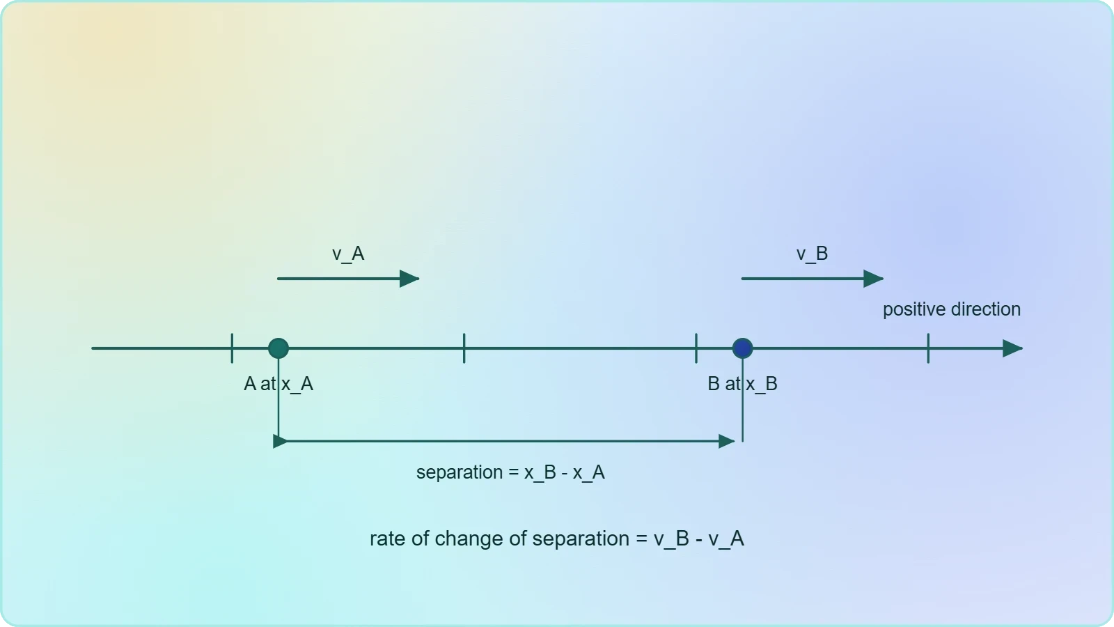
Consider two objects on a number line, one at position ##x_A## moving at ##v_A## and the other at ##x_B## moving at ##v_B##. The separation between them changes at a rate equal to the difference of their velocities, and this single statement generates every formula used below. Nothing more elaborate is required for the exam-level problems this course targets.

Why the Reference Frame Simplifies Everything

Choosing a moving reference frame is the most powerful simplification available to a problem-solver. By mentally riding alongside one object, the solver freezes that object and lets the other move at the relative speed. The problem collapses from two moving bodies to one, and the familiar tools of the previous lesson apply directly.

This frame-shifting habit also guards against the most common error in the topic: adding speeds when they should be subtracted, or the reverse. Once the frame is fixed, the direction of the remaining motion is unambiguous, and the arithmetic follows naturally without guesswork or memorised rules.

Objects Moving in Opposite Directions

When two bodies approach each other head-on, the gap between them shrinks faster than either body moves alone. Each contributes its own speed to the closing rate, so the relative speed equals the sum of the individual speeds. This additive behaviour is intuitive: two people walking toward each other cover the separating distance twice as quickly as one alone.

Opposite-direction motion appears constantly in exam papers, from two trains on parallel tracks to two runners on a circular track starting from opposite ends. Recognising the configuration is the first step; the second is applying the sum cleanly and converting units consistently before any arithmetic begins. The formula below captures the entire relationship.

The Additive Formula and Its Derivation

Let the two bodies be separated by a distance ##d## and moving toward each other at speeds ##u## and ##v##. In one unit of time, the first covers ##u## and the second covers ##v##, so the gap closes by ##u + v##. The time to meet is therefore the initial separation divided by this combined rate.

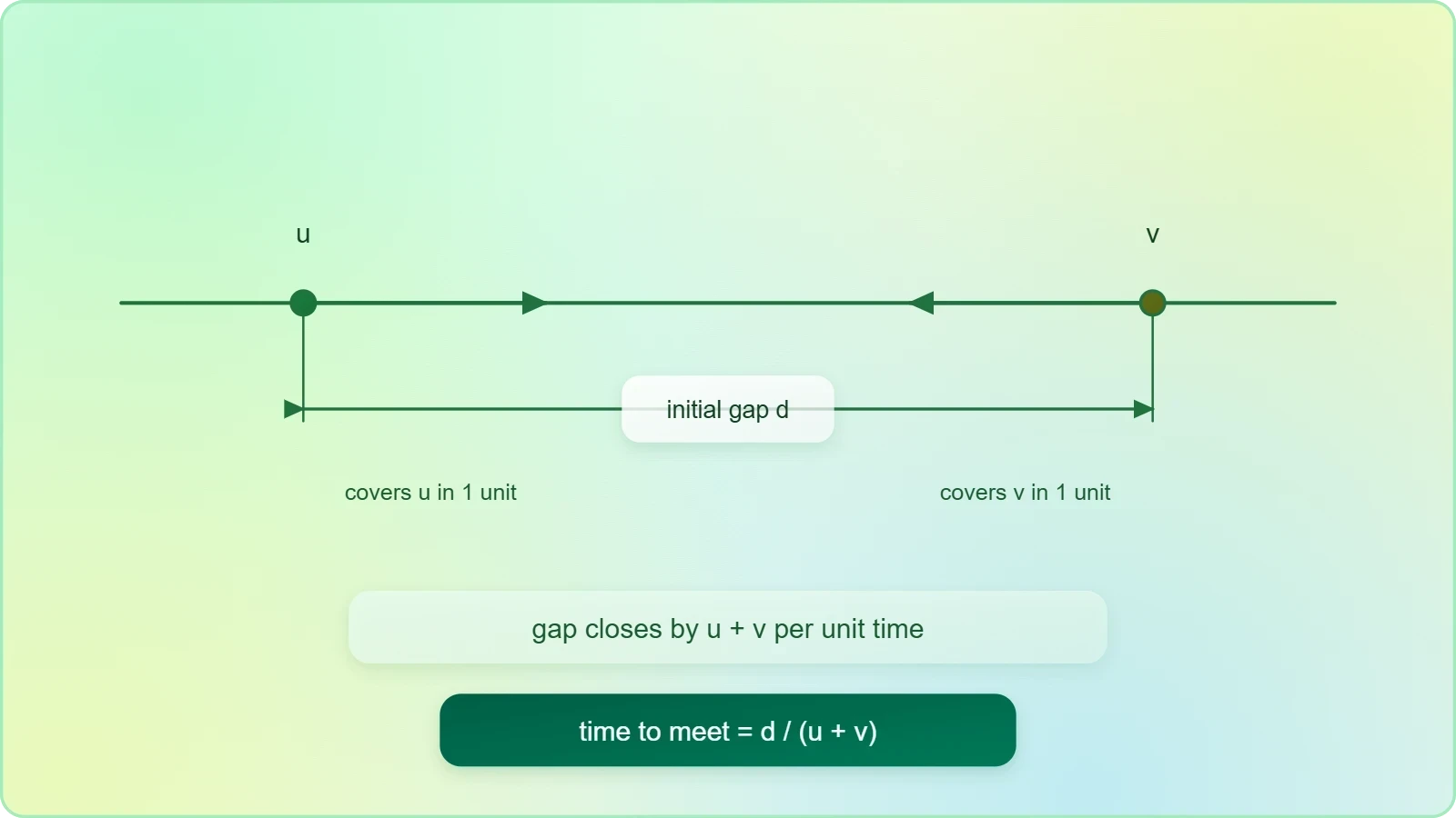
The derivation is short but worth internalising, because it generalises immediately. If the bodies start from the same point and move apart in opposite directions, the same sum governs how quickly the separation grows, and the time to reach a given separation is again ##d/(u+v)##. One formula, two mirror-image applications.

Worked Illustration with Two Travellers

Suppose two towns lie 240 kilometres apart, and two travellers depart simultaneously toward each other at 50 and 70 kilometres per hour. The closing speed is 120 kilometres per hour, so they meet after two hours. At that moment, the slower traveller has covered 100 kilometres and the faster 140, which together account for the full distance.

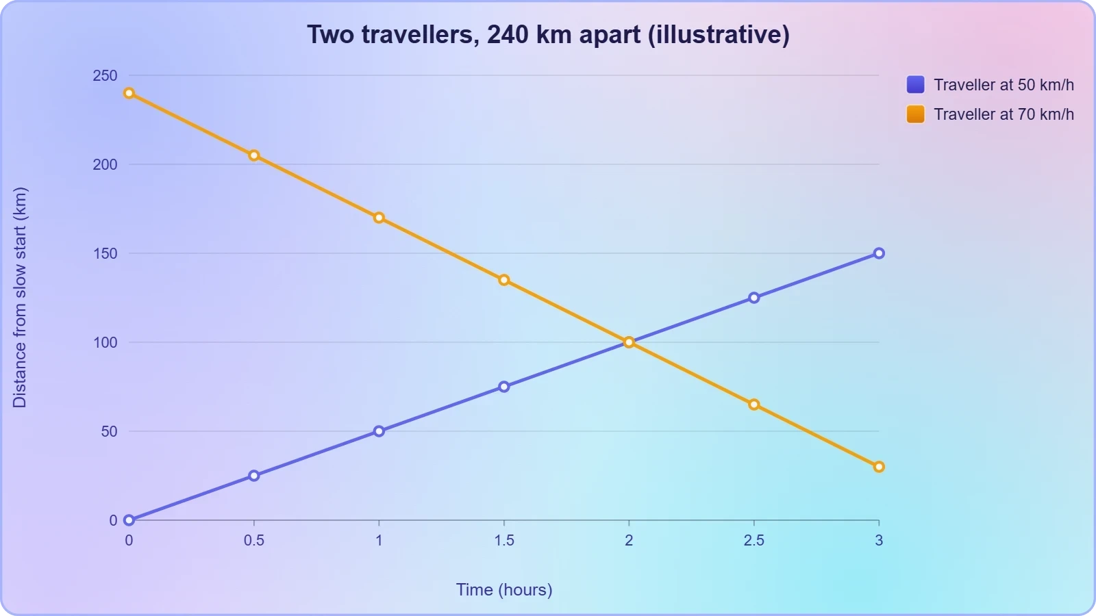
Notice how the meeting point is not the midpoint; it sits closer to the slower traveller's origin, in proportion to the speeds. Examiners frequently ask for this meeting distance rather than the time, and the proportional reasoning above answers it without a second calculation. The table below consolidates the opposite-direction relationships for quick revision.

Objects Moving in the Same Direction

Same-direction motion behaves very differently, and this is where careless candidates lose marks. When two bodies travel the same way, the faster one gains on the slower only at the difference of their speeds. The gap closes slowly, and if the speeds are equal, it never closes at all. Subtraction, not addition, is the operative rule.

The intuition is straightforward once framed correctly. Imagine walking behind a friend who moves slightly faster; the distance between you grows, but only by the small excess of their pace over yours. The absolute speeds are large, yet the relative motion is modest. Examiners love this contrast because it punishes mechanical formula application.

The Subtractive Formula and Overtaking

If a faster body at speed ##u## trails a slower one at speed ##v## by a lead ##d##, the gain per unit time is ##u - v##. Overtaking occurs when the accumulated gain equals the initial lead, giving the catch-up time below. The same expression answers how long a pursuer needs to close any head start.

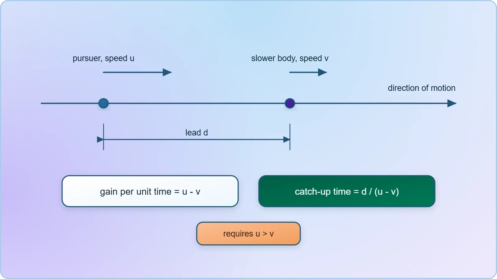
Two conditions deserve emphasis. First, the formula requires ##u > v##; if the pursuer is not genuinely faster, no overtaking ever happens and the problem is a trap. Second, the lead ##d## must be measured at the same instant for both bodies, otherwise the arithmetic silently incorporates an error that no amount of checking will reveal.

Reading the Sign and the Direction

Treating one direction as positive and the other as negative turns both cases into a single rule: relative speed is the algebraic difference of velocities. Opposite directions then produce a sum automatically, because subtracting a negative adds. This sign discipline removes the need to remember two separate formulas under exam pressure.

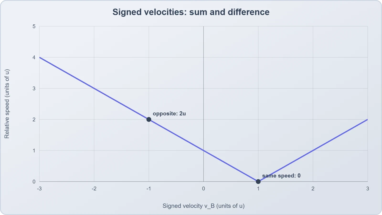
Practising with signed velocities also prepares candidates for the train problems ahead, where a train and a person may move the same way or against each other. The habit of assigning a positive direction first, then writing every velocity with its sign, is the most reliable defence against the classic addition-subtraction confusion.

Unit Discipline and Conversion Before Calculation

Relative speed problems fail more often on units than on concepts. A speed in kilometres per hour paired with a distance in metres, or a time in minutes, produces nonsense unless converted first. The safe habit is to fix a single system before touching the formula: metres and seconds, or kilometres and hours, never a mixture of both.

The conversion factor between the two common systems is the workhorse of this topic. Multiplying a kilometre-per-hour figure by five-eighteenths yields metres per second, while the reciprocal conversion multiplies by eighteen-fifths. Candidates who rehearse these two factors until automatic eliminate an entire class of avoidable errors from their solutions.

The Conversion Factors in Practice

Applied to relative speed, the conversion must be performed on the combined rate, not on the individual speeds separately, whenever the two are already summed. Doing it the other way usually works but invites arithmetic slips. The cleaner sequence is to add or subtract first, then convert the single resulting figure once.

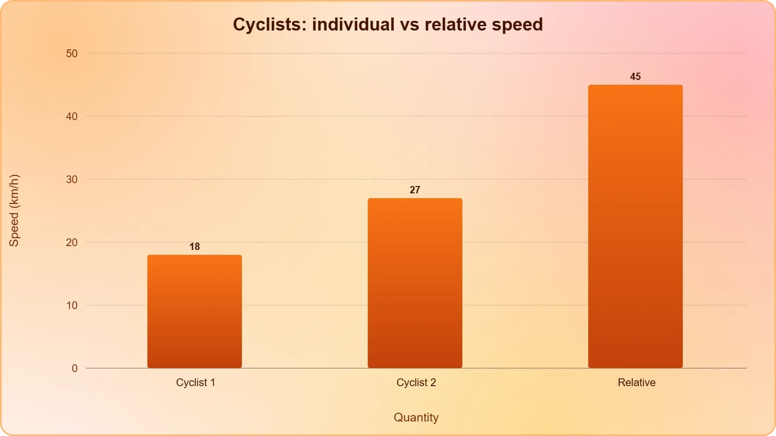
Consider two cyclists approaching at 18 and 27 kilometres per hour. Their relative speed is 45 kilometres per hour, which converts to 12.5 metres per second. If they are 500 metres apart, they meet in forty seconds. Converting first and adding later would have produced the same answer, but with more intermediate figures to mistype.

A Short Conversion Routine

Encoding the routine as a small script makes the discipline concrete and mirrors how computational candidates verify answers during practice. The function below accepts two speeds and a direction flag, returning the relative speed in the requested unit. It is deliberately simple, because clarity matters more than cleverness in exam preparation.

def relative_speed(u, v, same_direction=True, unit="kmh"):
    """Return relative speed of two bodies moving along one line."""
    rate = abs(u - v) if same_direction else (u + v)
    if unit == "ms":
        rate = rate * 5 / 18
    return rate

# Two cyclists approaching head-on
print(relative_speed(18, 27, same_direction=False))   # 45 km/h
print(relative_speed(18, 27, same_direction=False, unit="ms"))  # 12.5 m/s

Applying Relative Speed to Real Scenarios

Textbook formulas acquire meaning only when attached to situations a candidate can visualise. Two friends cycling toward each other on a straight road, a police jeep pursuing a speeding car, a swimmer working upstream against a current: each is a relative-speed problem in disguise. Recognising the disguise is the transferable skill this section cultivates.

The scenarios below deliberately avoid trains, which belong to the next lesson, and avoid the averaging logic of the previous one. What remains is the pure two-body interaction, examined from several angles so that the underlying structure becomes visible beneath the surface details of each story.

Pursuit, Approach, and the River Current

A river problem is relative speed wearing natural clothing. A boat's speed in still water combines with the current's speed: downstream the two add, upstream they subtract. A boat capable of 10 kilometres per hour in still water meets a 2 kilometre per hour current and achieves 12 downstream but only 8 upstream, a difference examiners probe constantly.

Pursuit problems follow the subtractive rule with a head start. If a car passes a checkpoint at 60 kilometres per hour and a second car leaves the same point twenty minutes later at 80, the lead at departure is 20 kilometres. The closing rate is 20 kilometres per hour, so the second car catches up in exactly one hour.

Circular Tracks and Meeting Points

On a circular track, relative speed determines how often runners meet. Two runners circling in opposite directions meet whenever their combined distance equals one lap, so the meeting interval is the track length divided by the sum of their speeds. Same-direction runners meet when the faster has gained exactly one full lap.

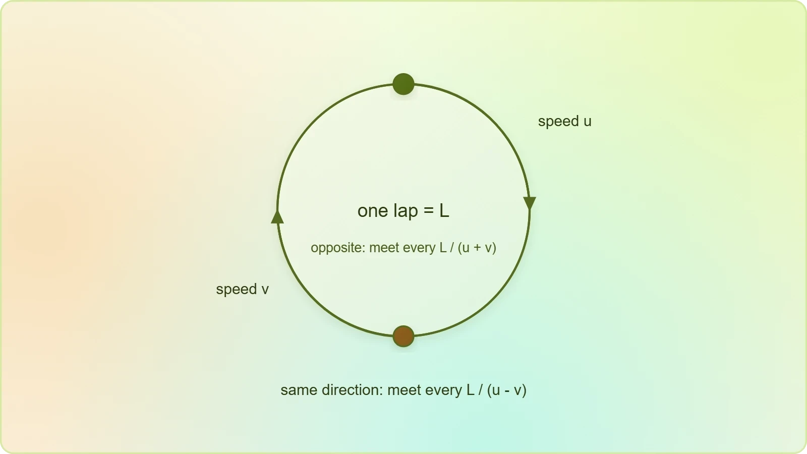
This lap-based reasoning generalises elegantly: the ##n##-th meeting occurs when the relative distance equals ##n## laps. Candidates who grasp this see circular-track questions as straightforward extensions of the linear case rather than a separate topic requiring fresh memorisation. The table below records the standard circular-track results.

Diagnosing Errors and Building Exam Technique

Most lost marks in this topic trace to a small set of recurring mistakes, and naming them explicitly is the fastest route to eliminating them. Adding speeds when the bodies move the same way, forgetting to convert units, and misreading a head start as a distance rather than a time are the three most frequent culprits. Each has a simple antidote.

Beyond error avoidance, technique matters. Drawing a quick sketch of the two bodies, marking directions with arrows, and writing the relative speed before any other quantity turns a word problem into a diagram problem. The sketch costs fifteen seconds and routinely saves a minute of confused algebra, especially under timed conditions.

Common Traps and Their Antidotes

The head-start trap deserves particular attention. A statement that one body starts twenty minutes later is a time, not a distance, and must be converted into a lead using the first body's speed. Candidates who treat the twenty minutes as a distance produce answers that are dimensionally wrong yet superficially plausible, which makes the error hard to spot.

Another trap hides in questions about bodies of negligible length, such as people or cyclists, versus bodies with length, such as trains. This lesson deliberately restricts itself to the former; the moment length enters, the problem shifts into the territory of the next lesson, where crossing times replace simple meeting times.

A Practice Set for Consolidation

Three short problems consolidate the lesson. First, two walkers 36 kilometres apart approach at 5 and 7 kilometres per hour; find the meeting time. Second, a runner at 12 kilometres per hour chases one at 9 with a 6 kilometre lead; find the catch-up time. Third, two boats cross a 2 kilometre river at 8 and 6 kilometres per hour in still water with a 2 kilometre per hour current; compare their crossing times.

Worked answers follow the same pattern each time: identify the configuration, compute the relative speed, convert units if needed, then divide the separation by that rate. Repeating the pattern across varied contexts is what converts understanding into speed, and speed is precisely what the examination rewards.

Preparing the Ground for Train Problems

The next lesson introduces bodies with measurable length, and the transition is smoother than it first appears. A train crossing a pole is a point meeting a moving segment; a train crossing a platform is a segment meeting a stationary segment. Both reduce to relative speed once the relevant distance is identified correctly.

What changes is the distance, not the rate. Instead of the gap between two points, the relevant distance becomes the sum of the lengths involved, or the length of the moving body alone. Candidates who arrive at that lesson fluent in relative speed spend their effort on identifying distances rather than relearning rates.

Bridging the Two Topics

A useful preview: when a train of length ##L## passes a stationary pole, the distance travelled is ##L##, and the time is ##L## divided by the train's speed. When it passes a platform of length ##P##, the distance becomes ##L + P##. The rate is unchanged; only the numerator grows.

When two trains cross each other, the relative speed returns in full force, additive for opposite directions and subtractive for the same. The distance in that case is the sum of the two lengths. Every element of the coming lesson is therefore already familiar, merely recombined in a new configuration.

Consolidation Checklist Before Moving On

Before proceeding, confirm four competencies. Can you state the relative speed for both configurations without hesitation? Can you convert between kilometres per hour and metres per second fluently? Can you translate a time-based head start into a distance lead? Can you sketch a problem and mark directions before calculating?

Affirmative answers to all four mean the foundation is secure. Anything less warrants a return to the worked examples above, since the train problems ahead assume these skills rather than teaching them. The table below summarises the readiness criteria in a form suitable for a final self-audit.